icomb

Introduction

Forecast reconciliation is used to make forecasts coherent across a hierarchy or grouped structure. In the Australian tourism data, trips can be aggregated by State, by Purpose, and by their combinations. If forecasts are produced independently for each series, the results will generally not add up correctly across the structure.

This vignette demonstrates a workflow that goes a step further than reconciliation alone. Alongside coherent forecasts, we also examine which series are selected by icomb, and whether those series exhibit distinctive time series characteristics.

The analysis proceeds in four stages:

1. construct a grouped tourism structure

2. fit base forecast models and reconcile the forecasts

3. extract series inclusion information from icomb

4. relate inclusion of series to feature-based summaries or accuracy of the series.

Packages

library(dplyr)
library(tsibble)
library(fable)
library(icomb)
library(feasts)
library(ggplot2)
library(plotly)

Workflow

Building a grouped tourism structure

We begin with the tourism dataset available in the tsibble package and aggregate trips across the State and Purpose dimensions to create a simple grouped structure.

tourism_gts <- tourism |>
  aggregate_key(State * Purpose,
                Trips = sum(Trips))
tourism_gts
#> # A tsibble: 3,600 x 4 [1Q]
#> # Key:       State, Purpose [45]
#> Loading required namespace: crayon
#>    Quarter State        Purpose       Trips
#>      <qtr> <chr*>       <chr*>        <dbl>
#>  1 1998 Q1 <aggregated> <aggregated> 23182.
#>  2 1998 Q2 <aggregated> <aggregated> 20323.
#>  3 1998 Q3 <aggregated> <aggregated> 19827.
#>  4 1998 Q4 <aggregated> <aggregated> 20830.
#>  5 1999 Q1 <aggregated> <aggregated> 22087.
#>  6 1999 Q2 <aggregated> <aggregated> 21458.
#>  7 1999 Q3 <aggregated> <aggregated> 19914.
#>  8 1999 Q4 <aggregated> <aggregated> 20028.
#>  9 2000 Q1 <aggregated> <aggregated> 22339.
#> 10 2000 Q2 <aggregated> <aggregated> 19941.
#> # ℹ 3,590 more rows

This grouped structure contains the total, the marginal aggregates (i.e., state level aggregates and purpose level aggregates), and the bottom-level series defined by each State and Purpose combination. These connected series form a natural setting for forecast reconciliation.

Fitting base forecasts

We next fit an ETS model to every series in the grouped structure. You can fit any other univariate models or multivariate model(s).

fit <- tourism_gts |>
  model(base = ETS(Trips))
fit
#> # A mable: 45 x 3
#> # Key:     State, Purpose [45]
#>    State           Purpose              base
#>    <chr*>          <chr*>            <model>
#>  1 ACT             Business     <ETS(M,N,M)>
#>  2 ACT             Holiday      <ETS(M,N,A)>
#>  3 ACT             Other        <ETS(M,N,N)>
#>  4 ACT             Visiting     <ETS(M,N,N)>
#>  5 ACT             <aggregated> <ETS(M,A,N)>
#>  6 New South Wales Business     <ETS(M,N,A)>
#>  7 New South Wales Holiday      <ETS(M,N,A)>
#>  8 New South Wales Other        <ETS(A,N,N)>
#>  9 New South Wales Visiting     <ETS(A,N,A)>
#> 10 New South Wales <aggregated> <ETS(A,N,A)>
#> # ℹ 35 more rows

These are the base forecasts. Since each series is modeled independently, the forecasts are not guaranteed to be coherent with the aggregation constraints.

Reconciling base forecasts

We reconcile the base forecasts using two methods.

• ols: MinT reconciliation with \mathbf{W}_h \propto \mathbf{I}

• icomb: the icomb reconciliation method with group lasso penalty (default option)

fit_recon <- fit |>
  reconcile(
    ols = min_trace(base, method = "ols"),
    icomb = icomb(base, train_size = 55)
  )
fit_recon
#> # A mable: 45 x 5
#> # Key:     State, Purpose [45]
#>    State           Purpose              base ols          icomb       
#>    <chr*>          <chr*>            <model> <model>      <model>     
#>  1 ACT             Business     <ETS(M,N,M)> <ETS(M,N,M)> <ETS(M,N,M)>
#>  2 ACT             Holiday      <ETS(M,N,A)> <ETS(M,N,A)> <ETS(M,N,A)>
#>  3 ACT             Other        <ETS(M,N,N)> <ETS(M,N,N)> <ETS(M,N,N)>
#>  4 ACT             Visiting     <ETS(M,N,N)> <ETS(M,N,N)> <ETS(M,N,N)>
#>  5 ACT             <aggregated> <ETS(M,A,N)> <ETS(M,A,N)> <ETS(M,A,N)>
#>  6 New South Wales Business     <ETS(M,N,A)> <ETS(M,N,A)> <ETS(M,N,A)>
#>  7 New South Wales Holiday      <ETS(M,N,A)> <ETS(M,N,A)> <ETS(M,N,A)>
#>  8 New South Wales Other        <ETS(A,N,N)> <ETS(A,N,N)> <ETS(A,N,N)>
#>  9 New South Wales Visiting     <ETS(A,N,A)> <ETS(A,N,A)> <ETS(A,N,A)>
#> 10 New South Wales <aggregated> <ETS(A,N,A)> <ETS(A,N,A)> <ETS(A,N,A)>
#> # ℹ 35 more rows

The icomb method with group lasso penalty is especially useful for exploratory analysis because it allows us to study which series are included in the information combination process.

Inspecting reconciliation output

To investigate the behavior of icomb, we glance the reconciliation results which provides .included variable indicating which series are selected by icomb for reconciliation.

glance_output <- fit_recon |>
  glance()
glance_output
#> # A tibble: 135 × 12
#>    State  Purpose  .model sigma2 log_lik   AIC  AICc   BIC   MSE  AMSE
#>    <chr*> <chr*>   <chr>   <dbl>   <dbl> <dbl> <dbl> <dbl> <dbl> <dbl>
#>  1 ACT    Business base   0.0540   -453.  919.  921.  936. 1069. 1071.
#>  2 ACT    Business ols    0.0540   -453.  919.  921.  936. 1069. 1071.
#>  3 ACT    Business icomb  0.0540   -453.  919.  921.  936. 1069. 1071.
#>  4 ACT    Holiday  base   0.0680   -463.  940.  941.  956. 1509. 1538.
#>  5 ACT    Holiday  ols    0.0680   -463.  940.  941.  956. 1509. 1538.
#>  6 ACT    Holiday  icomb  0.0680   -463.  940.  941.  956. 1509. 1538.
#>  7 ACT    Other    base   0.202    -376.  759.  759.  766.  154.  156.
#>  8 ACT    Other    ols    0.202    -376.  759.  759.  766.  154.  156.
#>  9 ACT    Other    icomb  0.202    -376.  759.  759.  766.  154.  156.
#> 10 ACT    Visiting base   0.0305   -450.  905.  905.  912.  965. 1038.
#> # ℹ 125 more rows
#> # ℹ 2 more variables: MAE <dbl>, .included <lgl>

Computing time series features

To describe the series in the structure statistically, we compute a broad collection of features using feasts.

tourism_features <- tourism_gts |>
  features(Trips, feature_set(pkgs = "feasts"))
tourism_features
#> # A tibble: 45 × 50
#>    State           Purpose      trend_strength seasonal_strength_year
#>    <chr*>          <chr*>                <dbl>                  <dbl>
#>  1 ACT             Business              0.526                  0.405
#>  2 ACT             Holiday               0.603                  0.453
#>  3 ACT             Other                 0.502                  0.254
#>  4 ACT             Visiting              0.600                  0.136
#>  5 ACT             <aggregated>          0.725                  0.184
#>  6 New South Wales Business              0.785                  0.635
#>  7 New South Wales Holiday               0.750                  0.891
#>  8 New South Wales Other                 0.874                  0.303
#>  9 New South Wales Visiting              0.831                  0.733
#> 10 New South Wales <aggregated>          0.908                  0.760
#> # ℹ 35 more rows
#> # ℹ 46 more variables: seasonal_peak_year <dbl>, seasonal_trough_year <dbl>,
#> #   spikiness <dbl>, linearity <dbl>, curvature <dbl>, stl_e_acf1 <dbl>,
#> #   stl_e_acf10 <dbl>, acf1 <dbl>, acf10 <dbl>, diff1_acf1 <dbl>,
#> #   diff1_acf10 <dbl>, diff2_acf1 <dbl>, diff2_acf10 <dbl>, season_acf1 <dbl>,
#> #   pacf5 <dbl>, diff1_pacf5 <dbl>, diff2_pacf5 <dbl>, season_pacf <dbl>,
#> #   zero_run_mean <dbl>, nonzero_squared_cv <dbl>, zero_start_prop <dbl>, …

These features capture properties such as trend strength, seasonal strength, autocorrelation, linearity, and aspects of forecastability. See the online Forecasting: Principles and Practice textbook for a detailed description of these features.

Rather than inspecting dozens of features one at a time, it is often useful to summarize them in a smaller feature space.

Reducing the feature space with PCA

We use principal component analysis (PCA) to obtain a low-dimensional representation of the features.

pcs <- tourism_features |>
  select(-State, -Purpose, -zero_run_mean, -zero_start_prop, -zero_end_prop) |>
  prcomp(scale = TRUE) |>
  broom::augment(tourism_features)
pcs
#> # A tibble: 45 × 96
#>    .rownames State           Purpose      trend_strength seasonal_strength_year
#>    <chr>     <chr*>          <chr*>                <dbl>                  <dbl>
#>  1 1         ACT             Business              0.526                  0.405
#>  2 2         ACT             Holiday               0.603                  0.453
#>  3 3         ACT             Other                 0.502                  0.254
#>  4 4         ACT             Visiting              0.600                  0.136
#>  5 5         ACT             <aggregated>          0.725                  0.184
#>  6 6         New South Wales Business              0.785                  0.635
#>  7 7         New South Wales Holiday               0.750                  0.891
#>  8 8         New South Wales Other                 0.874                  0.303
#>  9 9         New South Wales Visiting              0.831                  0.733
#> 10 10        New South Wales <aggregated>          0.908                  0.760
#> # ℹ 35 more rows
#> # ℹ 91 more variables: seasonal_peak_year <dbl>, seasonal_trough_year <dbl>,
#> #   spikiness <dbl>, linearity <dbl>, curvature <dbl>, stl_e_acf1 <dbl>,
#> #   stl_e_acf10 <dbl>, acf1 <dbl>, acf10 <dbl>, diff1_acf1 <dbl>,
#> #   diff1_acf10 <dbl>, diff2_acf1 <dbl>, diff2_acf10 <dbl>, season_acf1 <dbl>,
#> #   pacf5 <dbl>, diff1_pacf5 <dbl>, diff2_pacf5 <dbl>, season_pacf <dbl>,
#> #   zero_run_mean <dbl>, nonzero_squared_cv <dbl>, zero_start_prop <dbl>, …

The coordinates .fittedPC1 and .fittedPC2 summarize the dominant variation across the extracted series features.

Joining features, node inclusion, and accuracy

To compare statistical features with reconciliation behavior, we join together

• the PCA representation
• the node inclusion indicator from icomb, and
• base-model accuracy measures

all_info <- glance_output |>
  filter(.model == "icomb") |>
  select(State, Purpose, .included) |>
  full_join(pcs, by = c("State", "Purpose"))

all_info <- accuracy(fit) |>
  select(-.model, -.type) |>
  full_join(all_info, by = c("State", "Purpose"))
all_info
#> # A tibble: 45 × 105
#>    State        Purpose       ME  RMSE   MAE      MPE  MAPE  MASE RMSSE     ACF1
#>    <chr*>       <chr*>     <dbl> <dbl> <dbl>    <dbl> <dbl> <dbl> <dbl>    <dbl>
#>  1 ACT        … Business    4.90  32.7  26.7  -1.52   18.6  0.703 0.739  0.0312 
#>  2 ACT        … Holiday     3.63  38.9  28.5  -2.00   18.6  0.839 0.842  0.110  
#>  3 ACT        … Other       1.32  12.4  10.2 -16.0    42.6  0.789 0.773  0.0614 
#>  4 ACT        … Visiting    3.28  31.1  23.2  -0.622  12.2  0.684 0.704  0.0737 
#>  5 ACT        … <aggregat…  7.91  60.9  49.0   0.0964  9.75 0.709 0.697  0.0913 
#>  6 New South W… Business    9.69 128.  102.   -0.0675  8.10 0.785 0.789 -0.0967 
#>  7 New South W… Holiday     8.36 168.  136.   -0.0168  4.56 0.805 0.785  0.00534
#>  8 New South W… Other       5.91  41.4  34.9   0.0551 12.1  0.851 0.828 -0.0737 
#>  9 New South W… Visiting   13.9  151.  124.    0.202   5.21 0.696 0.699  0.0391 
#> 10 New South W… <aggregat… 32.6  300.  243.    0.268   3.53 0.731 0.725 -0.0306 
#> # ℹ 35 more rows
#> # ℹ 95 more variables: .included <lgl>, .rownames <chr>, trend_strength <dbl>,
#> #   seasonal_strength_year <dbl>, seasonal_peak_year <dbl>,
#> #   seasonal_trough_year <dbl>, spikiness <dbl>, linearity <dbl>,
#> #   curvature <dbl>, stl_e_acf1 <dbl>, stl_e_acf10 <dbl>, acf1 <dbl>,
#> #   acf10 <dbl>, diff1_acf1 <dbl>, diff1_acf10 <dbl>, diff2_acf1 <dbl>,
#> #   diff2_acf10 <dbl>, season_acf1 <dbl>, pacf5 <dbl>, diff1_pacf5 <dbl>, …

This gives a single data frame linking each series to its features, inclusion status, and forecast accuracy metrics.

Visualizing series inclusion in feature space

A useful first question is whether included and excluded series occupy different regions of the feature space.

tourism_viz <- all_info |>
  ggplot(aes(
    x = .fittedPC1,
    y = .fittedPC2,
    colour = .included,
    text = paste0(
      "PC1: ", round(.fittedPC1, 2), "<br>",
      "PC2: ", round(.fittedPC2, 2), "<br>",
      "State: ", State, "<br>",
      "Purpose: ", Purpose, "<br>",
      "MAPE: ", round(MAPE, 2), "<br>",
      "RMSSE: ", round(RMSSE, 2), "<br>",
      "MASE: ", round(MASE, 2)
    )
  )) +
  geom_point()
tourism_viz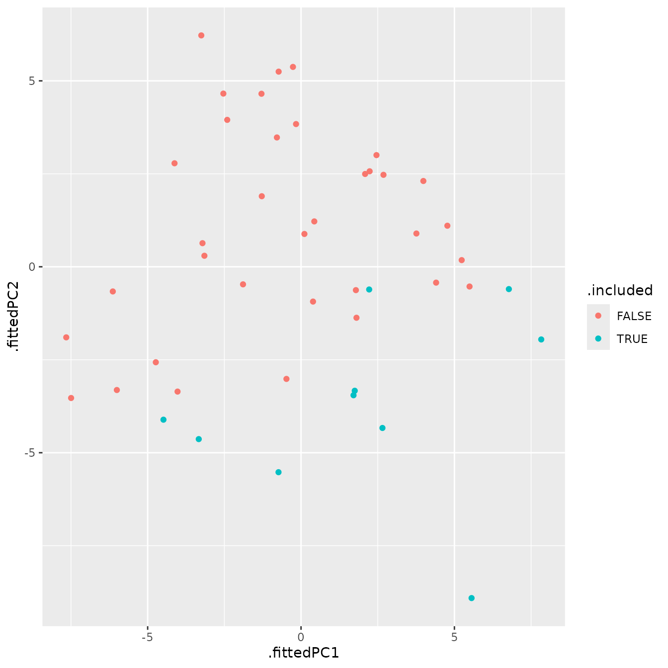

This plot provides a compact view of whether series inclusion in icomb is associated with the broad statistical profile of a series.

For interactive exploration in HTML output, the plot can also be converted with plotly.

tourism_viz |>
  ggplotly(tooltip = "text")

Examining interpretable features directly

While PCA is useful for summarizing many features at once, it is often easier to interpret individual features directly. Two especially common summaries are trend strength and annual seasonal strength.

tourism_feature_plot <- all_info |>
  ggplot(aes(
    x = trend_strength,
    y = seasonal_strength_year,
    colour = .included,
    text = paste0(
      "Trend_strength: ", round(trend_strength, 2), "<br>",
      "Seasonal_strength_year: ", round(seasonal_strength_year, 2), "<br>",
      "State: ", State, "<br>",
      "Purpose: ", Purpose, "<br>"
    )
  )) +
  geom_point()
tourism_feature_plot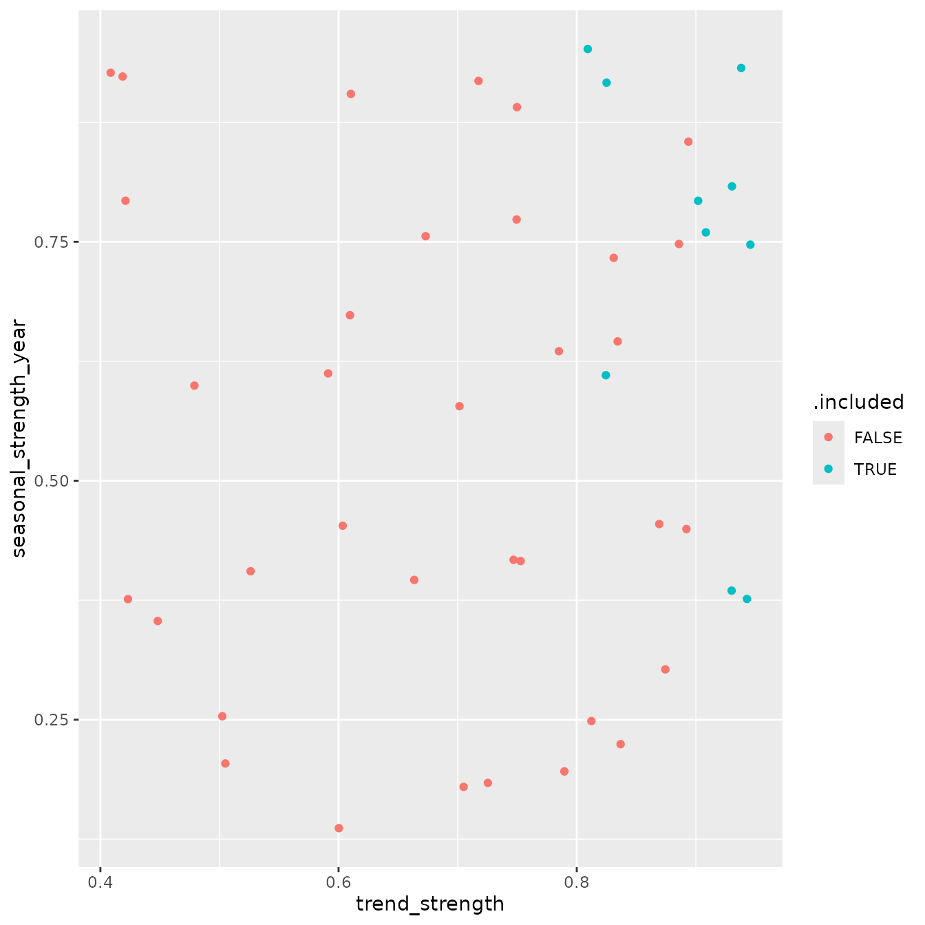

This plot helps assess whether included series tend to be more strongly trended, more seasonal, or broadly similar to excluded series.

An interactive version can also be produced

tourism_feature_plot |>
  ggplotly(tooltip = "text")

Comparing behavior across travel purpose

The relationship between structure and inclusion of series may differ by travel purpose. To explore this, we facet the trend-seasonality display by Purpose.

tourism_purpose_plot <- all_info |>
  ggplot(aes(
    x = trend_strength,
    y = seasonal_strength_year,
    colour = .included,
    text = paste0(
      "State: ", State, "<br>",
      "Purpose: ", Purpose, "<br>")
  )) +
  geom_point() +
  facet_wrap(vars(Purpose))
tourism_purpose_plot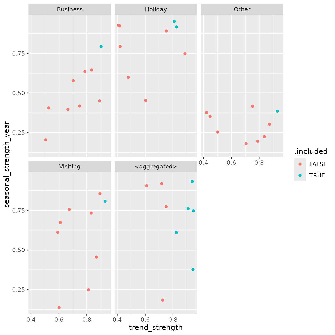

An interactive version can also be produced when desired.

tourism_purpose_plot |>
  ggplotly(text = "text")

Interpreting the results

This workflow makes it possible to ask questions such as:

• Do included series tend to be more regular or more forecastable?

• Are highly seasonal series more likely to be selected by icomb?

• Is inclusion associated with stronger or weaker base forecast accuracy?

• Do patterns differ systematically across purpose groups?

The answers will depend on the data and the implementation details of icomb, but the framework provides a practical way to connect reconciliation output with interpretable series characteristics.

Beyond summing constraints

The reconciliation methods discussed above are not limited to simple summation constraints. In general, both MinT based approaches and information combination methods can accommodate any linear constraints across a system of time series.

At present, the min_trace() implementation in fabletools is restricted to summing constraints. The icomb() approach, however, is more flexible and can be used in settings where the aggregation structure is defined differently.

Using averages instead of sums

As an illustration, suppose the structure is defined in terms of averages rather than totals. We can construct such a grouped structure by aggregating using mean() instead of sum().

tourism_avg_gts <- tourism_gts |>
  filter(!is_aggregated(State), !is_aggregated(Purpose)) |>
  aggregate_key(State * Purpose,
                Trips = mean(Trips))

We then fit and reconcile forecasts in the usual way.

fc <- tourism_avg_gts |>
  model(base = ETS(Trips)) |>
  reconcile(icomb = icomb(base, train_size = 55)) |>
  forecast()

To verify coherence under this alternative structure, we can recompute the averages from the bottom-level forecasts and compare them with the reconciled values.

fc |>
  filter(!is_aggregated(State), !is_aggregated(Purpose), .model == "icomb") |>
  aggregate_key(State * Purpose,
                mean_fc = mean(.mean)) |>
  full_join(fc |> filter(.model == "icomb")) |>
  mutate(diff = mean_fc - .mean) |>
  pull(diff) |>
  range()
#> Joining with `by = join_by(Quarter, State, Purpose)`
#> [1] -4.547474e-13  9.094947e-13

The range of differences is close to zero.

Current limitations and extensions

The current implementation of aggregate_key() in fabletools does not yet support arbitrary weights, which limits direct construction of more general linear constraints. This is expected to be addressed in future releases.

In the meantime, for fully general linear constraints, a practical approach is to manually construct a tsibble containing all series in the desired structure and pass it directly to model(). This provides complete flexibility in defining relationships among the series.