Implements the Information Combination (IComb) method for forecast reconciliation, combining information from multiple base forecasts through a regression-based framework that can be estimated using penalized regression techniques. The penalty parameter is estimated using the rolling forecast origin cross-validation.
Usage
icomb(
  models,
  train_size,
  alpha = 1,
  standardize = FALSE,
  standardize_response = FALSE,
  intercept = TRUE,
  lambda = NULL,
  lambda_min_ratio = "expand",
  nlambda = 100,
  maxit = 1e+07,
  thresh = 1e-07,
  exact = TRUE
)
Arguments
- models
A column of models in a mable.
- train_size
The size of the initial training window.
- alpha
The elasticnet mixing parameter, with \(0 \leq \alpha \leq 1\). The penalty is defined as $$(1 - \alpha)/2\|B\|_2^2 + \alpha\|B\|_2$$
alpha = 1is the group lasso penalty, andalpha = 0is the ridge penalty.- standardize
Logical flag for
xvariable standardization, prior to fitting the model sequence. The coefficients are always returned on the original scale. Default isstandardize = FALSE.- standardize_response
This allows the user to standardize the response variables. Default is
standardize_response = FALSE.- intercept
Should intercepts be fitted (default = TRUE) or set to zero (FALSE).
- lambda
A user supplied
lambdasequence. Typical usage is to have the program compute its ownlambdasequence based onnlambdaandlambda_min_ratio. Supplying a value oflambdaoverrides this. Supply a decreasing sequence oflambdavalues.- lambda_min_ratio
The smallest value for
lambda, as a fraction oflambda_max(the data derived value for which all coefficients are zero).lambda_min_ratio = "expand"(default) sets the ratio as \(10^{-\lfloor \log_{10}(\lambda_{max})\rfloor-2}\) whereaslambda_min_ratio = "glmnet"sets the ratio to the value used in theglmnetpackage. Ifnobs < nvars, the default is0.01, otherwise1e-04.- nlambda
The number of lambda values. Default is 100.
- maxit
Maximum number of passes over the data for all lambda values. Default is \(10^7\).
- thresh
Convergence threshold for coordinate descent. Each inner coordinate-descent loop continues until the maximum change in the objective after any coefficient update is less than thresh times the null deviance. Defaults value is 1e-07.
- exact
A logical flag indicating whether to use a sequence of lambda values (from
lambda_maxtolambda_best) when fitting the final model on the entire dataset. The functions in theglmnetpackage are designed for efficiency by computing the entire regularization path (a sequence of lambda values) using "warm starts", which is often faster than computing a single fit. The default isTRUE.
Note
Missing values are removed prior to applying the information combination method.
The default value of lambda_min_ratio may result in very small values of \(\lambda\), which can increase computation time. It is
therefore recommended to choose this parameter according to the specific requirements of your application.
Parallel computing
The model fitting and icomb cross-validation procedure can be parallelized using the future package.
By specifying a future::plan() prior to model estimation or the reconciliation step,
the computations will be carried out according to the chosen future strategy.
Progress
Progress on the cross-validation procedure can be obtained by wrapping the code with progressr::with_progress().
Further customization on how progress is reported can be controlled using the progressr package.
References
Nguyen, M., Vahid, F., & Wickramasuriya, S. L. (2025). Hierarchical Forecasting: The Role of Information Combination (Working Paper No. 11/25). Department of Econometrics and Business Statistics, Monash University.
Examples
library(fable)
library(fabletools)
library(tsibble)
library(dplyr)
library(lubridate)
#>
#> Attaching package: ‘lubridate’
#> The following object is masked from ‘package:tsibble’:
#>
#> interval
#> The following objects are masked from ‘package:base’:
#>
#> date, intersect, setdiff, union
library(ggtime)
tourism_hts <- tourism |>
aggregate_key(State,
Trips = sum(Trips))
fit <- tourism_hts |>
model(base = ETS(Trips)) |>
reconcile(ols = min_trace(base, method = "ols"),
icomb = icomb(base, train_size = 75))
fit |>
forecast(h = "3 years")
#> # A fable: 324 x 5 [1Q]
#> # Key: State, .model [27]
#> State .model Quarter
#> <chr*> <chr> <qtr>
#> 1 ACT base 2018 Q1
#> 2 ACT base 2018 Q2
#> 3 ACT base 2018 Q3
#> 4 ACT base 2018 Q4
#> 5 ACT base 2019 Q1
#> 6 ACT base 2019 Q2
#> 7 ACT base 2019 Q3
#> 8 ACT base 2019 Q4
#> 9 ACT base 2020 Q1
#> 10 ACT base 2020 Q2
#> # ℹ 314 more rows
#> # ℹ 2 more variables: Trips <dist>, .mean <dbl>
# extracting results from icomb cross-validation
fit |>
pull(icomb) |>
attr("icombfit")
#> $fit
#>
#> Call: glmnet(x = fitted[, !xconst_var], y = actual, family = "mgaussian", alpha = alpha, lambda = lambda_subset, standardize = standardize, intercept = intercept, thresh = thresh, maxit = maxit, standardize.response = standardize_response)
#>
#> Df %Dev Lambda
#> 1 0 0.00 4531000
#> 2 1 24.92 3762000
#> 3 1 42.10 3123000
#> 4 1 53.94 2593000
#> 5 1 62.10 2152000
#> 6 1 67.72 1787000
#> 7 1 71.60 1484000
#> 8 1 74.27 1232000
#> 9 1 76.11 1023000
#> 10 1 77.38 849000
#> 11 1 78.26 704800
#> 12 1 78.86 585200
#> 13 1 79.28 485800
#> 14 1 79.56 403300
#> 15 1 79.76 334900
#> 16 1 79.90 278000
#> 17 1 79.99 230800
#> 18 1 80.06 191600
#> 19 2 81.22 159100
#> 20 3 82.24 132100
#> 21 3 83.04 109700
#> 22 3 83.60 91030
#> 23 3 84.01 75580
#> 24 3 84.30 62750
#> 25 3 84.51 52090
#> 26 3 84.67 43250
#> 27 4 84.86 35910
#>
#> $info
#> $info$lambda_info
#> lambda_max lambda_best lambda_best_idx
#> 4530797.06 35905.79 27.00
#>
#> $info$mse_info
#> [1] 4124792.9 3956253.8 3393614.9 2605054.8 1914522.8 1426734.5 1080698.3
#> [8] 834034.0 657247.5 529774.5 437245.8 369595.0 319749.5 282722.5
#> [15] 254984.3 234024.8 218050.2 205770.8 187132.4 170435.0 158126.4
#> [22] 149164.9 142587.8 137672.9 133927.0 131004.9 129573.2 134981.8
#> [29] 143439.9 152149.1 160537.4 168248.8 175042.9 182362.1 191025.9
#> [36] 199308.1 206071.9 211941.9 211988.5 201918.6 192264.6 187160.6
#> [43] 174851.8 163909.9 155651.1 149587.2 145158.5 141917.9 139530.9
#> [50] 137764.1 136457.0 135476.1 134759.6 134208.5 133860.9 133507.3
#> [57] 133419.5 132938.8 132982.0 132769.9 132614.1 132775.1 132607.4
#> [64] 132702.0 132620.2 132584.0 132584.3 132605.9 132622.1 132619.3
#> [71] 132606.3 132499.1 132504.2 132508.9 132512.8 132577.7 132567.9
#> [78] 132559.0 132550.5 132542.6 132535.0 132527.7 132520.7 132513.9
#> [85] 132507.3 132500.9 132494.8 132488.8 132483.1 132477.5 132472.1
#> [92] 132466.9 132461.9 132457.1 132452.4 132447.8 132443.5 132439.2
#> [99] 132435.1 132431.1
#>
#> $info$nnzeros
#> [1] 4
#>
#>
#> $coefs
#> y1 y2 y3 y4 y5
#> intercept -8.268047e+01 2071.06249460 -1.849262e+02 508.65433184 573.461521165
#> V1 0.000000e+00 0.00000000 0.000000e+00 0.00000000 0.000000000
#> V2 -8.864111e-04 0.07393857 -7.720577e-03 -0.03524504 0.006601113
#> V3 0.000000e+00 0.00000000 0.000000e+00 0.00000000 0.000000000
#> V4 3.875545e-02 -0.28882092 1.598517e-01 0.62511957 -0.117136025
#> V5 0.000000e+00 0.00000000 0.000000e+00 0.00000000 0.000000000
#> V6 0.000000e+00 0.00000000 0.000000e+00 0.00000000 0.000000000
#> V7 -1.712496e-02 0.03407251 -1.326398e-01 -0.22427645 0.053466921
#> V8 0.000000e+00 0.00000000 0.000000e+00 0.00000000 0.000000000
#> V9 2.325875e-02 0.26111472 2.204911e-02 0.12416708 0.054060207
#> y6 y7 y8 y9
#> intercept 157.789749315 -4.812849e+02 -1.847343e+03 7.147331e+02
#> V1 0.000000000 0.000000e+00 0.000000e+00 0.000000e+00
#> V2 -0.007549028 -3.519441e-03 -2.011996e-02 5.499223e-03
#> V3 0.000000000 0.000000e+00 0.000000e+00 0.000000e+00
#> V4 -0.155841312 -2.421887e-01 1.238690e-01 1.436088e-01
#> V5 0.000000000 0.000000e+00 0.000000e+00 0.000000e+00
#> V6 0.000000000 0.000000e+00 0.000000e+00 0.000000e+00
#> V7 0.177321141 4.391588e-01 -2.375915e-02 3.062190e-01
#> V8 0.000000000 0.000000e+00 0.000000e+00 0.000000e+00
#> V9 0.021413919 2.061507e-01 1.565233e-01 8.687378e-01
#>
# \donttest{
# Extracting probabilistic forecasts
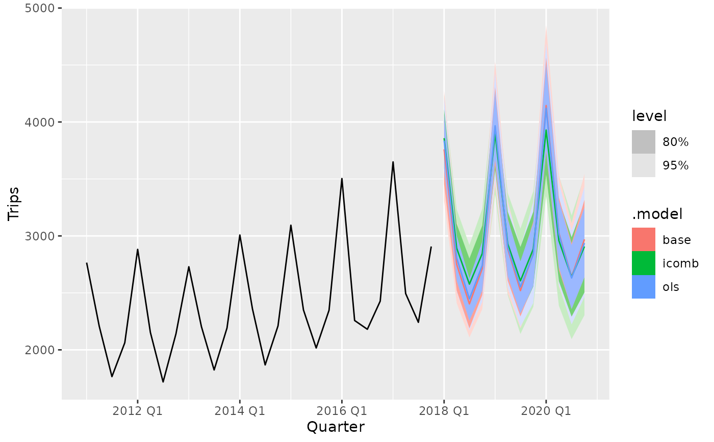
fit |>
forecast(h = "3 years", bootstrap = TRUE, times = 1000) |>
filter(State == "Victoria") |>
autoplot(filter(tourism_hts,
State == "Victoria", year(Quarter) > 2010))
 # grouped structure
tourism_gts <- tourism |>
aggregate_key(State * Purpose,
Trips = sum(Trips))
fit <- tourism_gts |>
model(base = ETS(Trips)) |>
reconcile(ols = min_trace(base, method = "ols"),
icomb = icomb(base, train_size = 75))
# Parallelizing cross-validation
library(future)
plan(multisession, workers = 2)
tourism_gts |>
model(base = ETS(Trips)) |>
reconcile(ols = min_trace(base, method = "ols"),
icomb = icomb(base, train_size = 75)) |>
forecast(h = "3 years")
#> Warning: There were 4 warnings in `mutate()`.
#> The first warning was:
#> ℹ In argument: `icomb = icomb(base, train_size = 75)`.
#> Caused by warning in `.resolve_control()`:
#> ! Passing 'thresh' to glmnet() is deprecated. Use control = list(thresh = ...) instead.
#> ℹ Run `dplyr::last_dplyr_warnings()` to see the 3 remaining warnings.
#> # A fable: 1,620 x 6 [1Q]
#> # Key: State, Purpose, .model [135]
#> State Purpose .model Quarter
#> <chr*> <chr*> <chr> <qtr>
#> 1 ACT Business base 2018 Q1
#> 2 ACT Business base 2018 Q2
#> 3 ACT Business base 2018 Q3
#> 4 ACT Business base 2018 Q4
#> 5 ACT Business base 2019 Q1
#> 6 ACT Business base 2019 Q2
#> 7 ACT Business base 2019 Q3
#> 8 ACT Business base 2019 Q4
#> 9 ACT Business base 2020 Q1
#> 10 ACT Business base 2020 Q2
#> # ℹ 1,610 more rows
#> # ℹ 2 more variables: Trips <dist>, .mean <dbl>
plan(sequential)
fit <- tourism_gts |>
model(base = ETS(Trips))
# progress
progressr::with_progress(
fit |>
reconcile(ols = min_trace(base, method = "ols"),
icomb = icomb(base, train_size = 35))
)
#> # A mable: 45 x 5
#> # Key: State, Purpose [45]
#> State Purpose base ols icomb
#> <chr*> <chr*> <model> <model> <model>
#> 1 ACT Business <ETS(M,N,M)> <ETS(M,N,M)> <ETS(M,N,M)>
#> 2 ACT Holiday <ETS(M,N,A)> <ETS(M,N,A)> <ETS(M,N,A)>
#> 3 ACT Other <ETS(M,N,N)> <ETS(M,N,N)> <ETS(M,N,N)>
#> 4 ACT Visiting <ETS(M,N,N)> <ETS(M,N,N)> <ETS(M,N,N)>
#> 5 ACT <aggregated> <ETS(M,A,N)> <ETS(M,A,N)> <ETS(M,A,N)>
#> 6 New South Wales Business <ETS(M,N,A)> <ETS(M,N,A)> <ETS(M,N,A)>
#> 7 New South Wales Holiday <ETS(M,N,A)> <ETS(M,N,A)> <ETS(M,N,A)>
#> 8 New South Wales Other <ETS(A,N,N)> <ETS(A,N,N)> <ETS(A,N,N)>
#> 9 New South Wales Visiting <ETS(A,N,A)> <ETS(A,N,A)> <ETS(A,N,A)>
#> 10 New South Wales <aggregated> <ETS(A,N,A)> <ETS(A,N,A)> <ETS(A,N,A)>
#> # ℹ 35 more rows
# }
# grouped structure
tourism_gts <- tourism |>
aggregate_key(State * Purpose,
Trips = sum(Trips))
fit <- tourism_gts |>
model(base = ETS(Trips)) |>
reconcile(ols = min_trace(base, method = "ols"),
icomb = icomb(base, train_size = 75))
# Parallelizing cross-validation
library(future)
plan(multisession, workers = 2)
tourism_gts |>
model(base = ETS(Trips)) |>
reconcile(ols = min_trace(base, method = "ols"),
icomb = icomb(base, train_size = 75)) |>
forecast(h = "3 years")
#> Warning: There were 4 warnings in `mutate()`.
#> The first warning was:
#> ℹ In argument: `icomb = icomb(base, train_size = 75)`.
#> Caused by warning in `.resolve_control()`:
#> ! Passing 'thresh' to glmnet() is deprecated. Use control = list(thresh = ...) instead.
#> ℹ Run `dplyr::last_dplyr_warnings()` to see the 3 remaining warnings.
#> # A fable: 1,620 x 6 [1Q]
#> # Key: State, Purpose, .model [135]
#> State Purpose .model Quarter
#> <chr*> <chr*> <chr> <qtr>
#> 1 ACT Business base 2018 Q1
#> 2 ACT Business base 2018 Q2
#> 3 ACT Business base 2018 Q3
#> 4 ACT Business base 2018 Q4
#> 5 ACT Business base 2019 Q1
#> 6 ACT Business base 2019 Q2
#> 7 ACT Business base 2019 Q3
#> 8 ACT Business base 2019 Q4
#> 9 ACT Business base 2020 Q1
#> 10 ACT Business base 2020 Q2
#> # ℹ 1,610 more rows
#> # ℹ 2 more variables: Trips <dist>, .mean <dbl>
plan(sequential)
fit <- tourism_gts |>
model(base = ETS(Trips))
# progress
progressr::with_progress(
fit |>
reconcile(ols = min_trace(base, method = "ols"),
icomb = icomb(base, train_size = 35))
)
#> # A mable: 45 x 5
#> # Key: State, Purpose [45]
#> State Purpose base ols icomb
#> <chr*> <chr*> <model> <model> <model>
#> 1 ACT Business <ETS(M,N,M)> <ETS(M,N,M)> <ETS(M,N,M)>
#> 2 ACT Holiday <ETS(M,N,A)> <ETS(M,N,A)> <ETS(M,N,A)>
#> 3 ACT Other <ETS(M,N,N)> <ETS(M,N,N)> <ETS(M,N,N)>
#> 4 ACT Visiting <ETS(M,N,N)> <ETS(M,N,N)> <ETS(M,N,N)>
#> 5 ACT <aggregated> <ETS(M,A,N)> <ETS(M,A,N)> <ETS(M,A,N)>
#> 6 New South Wales Business <ETS(M,N,A)> <ETS(M,N,A)> <ETS(M,N,A)>
#> 7 New South Wales Holiday <ETS(M,N,A)> <ETS(M,N,A)> <ETS(M,N,A)>
#> 8 New South Wales Other <ETS(A,N,N)> <ETS(A,N,N)> <ETS(A,N,N)>
#> 9 New South Wales Visiting <ETS(A,N,A)> <ETS(A,N,A)> <ETS(A,N,A)>
#> 10 New South Wales <aggregated> <ETS(A,N,A)> <ETS(A,N,A)> <ETS(A,N,A)>
#> # ℹ 35 more rows
# }